Avoiding overfitting is one of the key components of training a machine learning model. If the model is overfitting, its accuracy will be low. This happens because your model tries too hard to catch the noise in your training dataset. Your model becomes more adaptable as a result of learning such data points, but at the cost of overfitting.
Table of Contents
1 What is Overfitting?
A concept called overfitting happens when a machine learning model is restricted to the training set and is unable to perform effectively on unlabeled data.
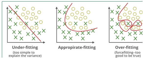
Grabbing the overfitting phenomenon requires an understanding of the concept of bias and variance balance. Utilizing cross-validation is one method of preventing overfitting because it helps in determining the parameters that work best for your model and in calculating the error over the test set. This essay will concentrate on a method that reduces overfitting while simultaneously improving model interpretability.
2 Regularization Techniques
Regularization is a method for reducing mistakes by properly fitting the function on the provided training set and avoiding overfitting.
The regularization methods most frequently employed are:
L1 regularization
L2 regularization
In this type of regression, the coefficient estimates are constrained, regularized, or shrunk in the direction of zero. To reduce the chance of overfitting, this strategy opposes learning a more sophisticated or flexible model.
This is a straightforward linear regression relationship. Here, Y stands for the learned relationship, and the coefficient estimates for various predictors or variables (X).
Let, Y ≈ β0 + β1X1 + β2X2 + …+ βpXp
The residual sum of squares or RSS, loss function is used during the fitting process. This loss function’s minimization is achieved by selecting the coefficients.
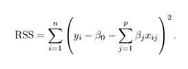
This will now modify the coefficients by your training data. The computed coefficients won’t generalize well to the subsequent data if there is noise in the training data. Regularization steps in at this point and shrinks or regularizes these learned estimates in the direction of zero.
3 How Does Regularization Work?
Two primary categories of regularization procedures are listed below:
- Ridge Regression
- Lasso Regression
3.1 Ridge Regression
The ridge regression depicted in the graphic above shows how the RSS is changed by including the shrinkage quantity. Currently, this function is minimized to estimate the coefficients. The tuning parameter, in this case, determines how much we want to penalize our model’s flexibility. If we want to reduce the size of the above function, then the coefficients of a model that represents an improvement in flexibility must be minimal.

This method does this by limiting the upward trend of coefficients. The estimated associations of each variable with the response have been shrunk, except for the intercept 0. This intercept measures the response’s mean value when xi1 = xi2 =…= xip = 0.
The estimates generated by ridge regression will be equal to least squares estimates when = 0, as the penalty term has no impact at that point. However, the shrinkage penalty’s effect increases, and the estimations of the ridge regression coefficients get closer to zero.
As can be seen, choosing an appropriate value is crucial. Cross-validation is useful in this situation. The L2 norm refers to the coefficient estimates generated by this procedure.
The typical least squares method yields coefficients that are scale equivariant, meaning that if we multiply each input by c, the associated coefficients are scaled by a factor of 1/c. As a result, no matter how the predictor is scaled, the predictor and coefficient(Xjj) are multiplied.
Ridge regression, however, does not work like this, thus before running ridge regression, we must normalize the predictors or scale them to the same value. Use the below formula for it.

Understand What is Regression in Machine Learning by checking our latest blog at SLA.
3.2 Lasso Regression
Another form is the lasso, in which the previous function is minimized. It is evident that the only way this variation and ridge regression differ is in how they treat large coefficients. Instead of squares of, its penalty is |j|(modulus). This is referred to as the L1 norm in statistics.

Let’s examine the aforementioned techniques from a different angle. When the summation of squares of coefficients is less than or equal to s, ridge regression can be viewed as the solution of an equation.
Additionally, the Lasso can be viewed as an equation where the sum of the coefficients’ moduli is smaller than or equal to s. In this case, the constant s holds true regardless of the shrinkage factor’s value. Constrained functions are another name for these equations.
Consider a problem that has 2 parameters. Then, using the aforementioned method, the ridge regression is represented as s = 12 + s = 22. This suggests that for all points inside the circle defined by 12 + 22 s, ridge regression coefficients have the fewest RSS (loss functions).
Similarly, the equation becomes |1|+|2|s for lasso. This suggests that for all points inside the diamond defined by |1|+|2|s, lasso coefficients have the smallest RSS (loss function).
These equations are represented in the graphic below.
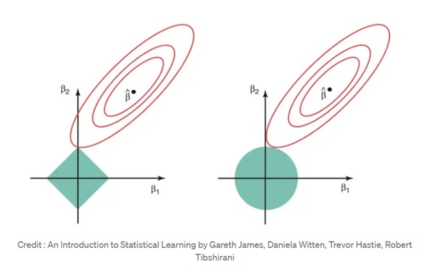
The aforementioned figure displays the contours for RSS together with the constraint functions (green regions) for lasso (left) and ridge regression (right) (red ellipse). The value of RSS is shared among points on the ellipse. The center of the ellipse will be contained by the green sections for very large values of s, making the coefficient estimates from both regression techniques equal to the least squares estimates.
In this instance, the first point at which an ellipse contacts the constraint zone provides estimates for the lasso and ridge regression coefficients. This intersection will typically not occur on an axis since ridge regression has a circular restriction with no sharp points, and as a result, the ridge regression coefficient estimates will exclusively be non-zero.
The ellipse will frequently cross the constraint zone at an axis because the lasso constraint contains corners at each of the axes. One of the coefficients will be equal to zero when this happens. Many of the coefficient estimations may be equal to zero at the same time in higher dimensions (when parameters are significantly more than 2).
This clarifies ridge regression’s obvious drawback, namely the model interpretability. The coefficients for the least significant predictors will decrease and eventually reach zero. However, it will never reduce them to zero.
In other words, all predictors will be there in the final model. When the tuning parameter is sufficiently big, the L1 penalty for the lasso, however, has the effect of driving some coefficient estimations to exactly equal zero. As a result, the lasso approach is stated to produce sparse models and also perform variable selection.
4 Comparison Between Ridge Regression and Lasso Regression

If there is significant collinearity between the independent variables, generally linear or polynomial regression will not succeed. Ridge regression can be utilized to address these issues. If we have more parameters than samples, that makes the problems easier to solve.
Enrich your AI skills by reading our blog on how can a DevOps team takes advantage of Artificial Intelligence.
5 What is the purpose of Regularization?
The variance of a basic least squares model means that it won’t generalize well to data sets other than its training set. Regularization dramatically lowers the model’s variance while maintaining or even increasing its bias. The impact on bias and variance is thus controlled by the tuning parameter, which is employed in the regularization procedures discussed above.
As the value increases, the coefficients’ values decrease, lowering the variance. Up to a degree, this rise is advantageous because it just reduces variance (avoiding overfitting), without losing any significant data features. After a specific value, however, the model starts to lose important traits, causing bias in the model and underfitting. Consequently, it’s crucial to make a good value decision.
Nothing more difficult is required to start the regularization procedure. It is a useful technique that can help increase the accuracy of your regression models. A well-liked library for implementing these algorithms is Scikit-Learn. With just a few lines of Python code, you can set up and run your model thanks to its amazing API.
6 Regularization Techniques in Machine Learning with Python
Let’s explore the Python implementation of regularization. We have used the Boston Housing Dataset to anticipate Boston housing prices using linear regression.
We begin by importing each of the required modules.
- import pandas as pd
- Import numpy as np
- Import matplotlib.pyplot as plt
- from sklearn import datasets
- from sklearn.model_selection import train_test_split
- from sklearn.linear_model import LinearRegression
The Boston Housing Dataset is then loaded from Sklearn’s datasets.
- boston_dataset = datasets.load_boston()
- After setting the columns and the target variable, we turn the dataset into a DataFrame.
- boston_pd = pd.DataFrame(boston_dataset.data)
- boston_pd.columns = boston_dataset.feature_names
- boston_pd_target = np.asarray(boston_dataset.target)
- boston_pd[‘House Price’] = pd.Series(boston_pd_target)
- X = boston_pd.iloc[:, :-1]
- Y = boston_pd.iloc[:, -1]
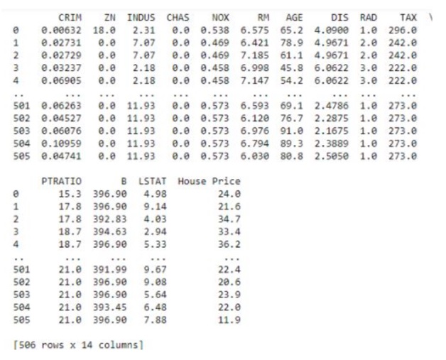
- print(boston_pd)
The housing dataset for Boston is displayed in the figure below.
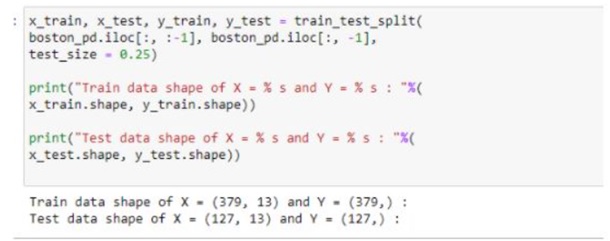
Our data was then split into training and testing sets.
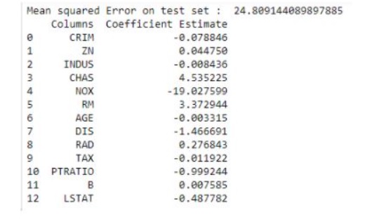
With their help, we can now train our linear regression model. To begin, we build our model and fit the data to it. We next make a prediction on the test set and use mean squared error to determine the error in our prediction. The coefficients of our linear regression model are then printed.
- lreg = LinearRegression()
- lreg.fit(x_train, y_train)
- lreg_y_pred = lreg.predict(x_test)
- mean_squared_error = np.mean((lreg_y_pred – y_test)**2)
- lreg_coefficient = pd.DataFrame()
- lreg_coefficient[“Columns”] = x_train.columns
- lreg_coefficient[“Coefficient Estimate”] = pd.Series(lreg.coef_)
- print(lreg_coefficient)
The following table contains the coefficients for our linear regression model.
Let’s plot the coefficient score right away.
- ifig, ax = plt.subplots(figsize = (20, 10))
- #now, color = [‘tab:gray’, ‘tab:blue’, ‘tab:orange’, ‘tab:green’, ‘tab:red’,
- ‘tab:purple’,
- ‘tab: brown’, ‘tab:pink’, ‘tab:pink’, ‘tab:gray’, ‘tab:olive’, ‘tab:cyan’, ‘tab:orange’,
- ‘tab:green’, ‘tab:blue’,
- ‘tab:olive’]
- ax.bar(lreg_coefficient[“Columns”], lreg_coefficient[‘Coefficient Estimate’], color = color)
- ax.spines[‘bottom’].set_position(‘zero’)
- plt.style.yse(‘ggplot’)
- plt.show()
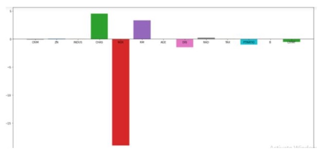
Let’s execute a Ridge regression now and visualize the new coefficients that we obtain.
- from sklearn.linear_model import Ridge
- ridgeR Ridge (alpha = 1)
- ridgeR.fit(x_train, y_train)
- y_pred = ridgeR.predict(x_test)
- mean_squared_error_ridge np.mean ((y_pred y_test)**2)
- print(“Mean squared error on test set”, mean_squared_error_ridge)
- ridge_coefficient pd.DataFrame()
- ridge_coefficient [“Columns”]= x_train.columns
- ridge_coefficient [ ‘Coefficient Estimate’] = pd.Series (ridgeR.coef_) print(ridge_coefficient)
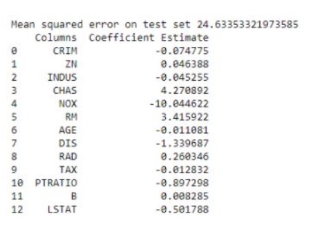
Let’s now plot the Ridge Regression model’s coefficient score.
- ifig, ax = plt.subplots(figsize (20, 10))
- So, color -[‘tab:gray’, ‘tab:blue’, ‘tab: orange’, ‘tab: green’, ‘tab:red’, ‘tab:purple’, ‘tab: brown”, ‘tab: pink’, ‘tab: gray’, ‘tab:olive’, ‘tab: cyan’, ‘tab: orange’, ‘tab: green’, ‘tab:blue’, ‘tab:olive’]
- ax.bar(lreg_coefficient [“Columns”],
- lreg_coefficient [‘Coefficient Estimate’], color – color)
- ax.spines[‘bottom’].set_position(‘zero’)
- plt.style.use(‘ggplot”)
- plt.show()
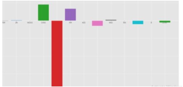
Now, Let’s execute the Lasso Regression and get its coefficients.
- from sklearn.linear_model import Lasso
- lasso = Lasso (alpha = 1)
- lasso.fit(x_train, y_train)
- y_pred1 = lasso.predict(x_test)
- mean_squared_error = np.mean ((y_pred1 y_test)**2)
- print(“Mean squared error on test set”, mean_squared_error)
- lasso_coeff = pd.DataFrame()
- lasso_coeff[“Columns”] = x_train.columns
- lasso_coeff[‘Coefficient Estimate’] = pd.Series (lasso.coef_)
- print (lasso_coeff)
7 Conclusion
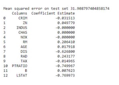
We were presented with the many ways that models might become unstable by being under or over-fitted in this article, Regularization in Machine Learning. After that, we looked at several regularization strategies for preventing over and under-fitting. Finally, a demo showed us how to apply regularization in Python. We hope you found this information about regularization helpful. Visit SLA today to learn more about the Machine Learning Course with IBM Certification.


