KNN Algorithm in Machine Learning

The k-nearest neighbors (kNN) method is a straightforward technique that may be applied to numerous practical issues in a variety of fields, including banking, healthcare, expert systems, and much more. What kNN is, how it functions, and how to use it in machine learning applications are all covered in this article.

Introduction to the kNN Algorithm

A supervised machine learning (ML) technique known as K-nearest neighbors (KNN) can be applied to classification and regression predicting issues. However, it is primarily employed in the industry for classification and forecasting problems. The next two characteristics would accurately describe KNN:

• • KNN is a lazy learning algorithm because it does not have a dedicated training phase and uses all of the data during classification for training.
  • KNN is also a non-parametric learning algorithm because it makes no assumptions about the underlying data.

K-Nearest Neighbor (KNN) Algorithm for Machine Learning

• • K-Nearest Neighbor is a simple machine learning algorithm based on the supervised learning method.
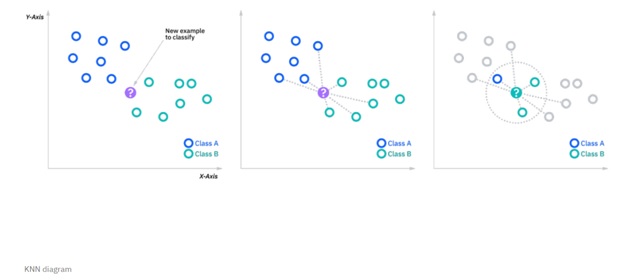
  • The K-NN algorithm assumes that the new and existing cases are comparable, and it assigns the new instance to the category that is most similar to the existing categories.
  • After all of the existing data has been stored, a new data point is classified using the K-NN algorithm based on similarity. This means that by employing the K-NN method, new data can be quickly and accurately classified.
  • Although the K-NN approach is most frequently employed for classification problems, it can also be utilized for regression.
  • Because K-NN is a non-parametric technique, no assumptions about the underlying data are made.
  • It is also known as a lazy learner algorithm since it saves the training dataset rather than learning from it immediately. Instead, it uses the dataset to perform an action when classifying data.
  • The KNN method simply saves the information during the training phase, and when it receives new data, it categorizes it into a category that is quite similar to the new data.

Join SLA for the Best Machine Learning Training in Chennai with IBM Certification

Why is a K-NN algorithm necessary for Machine Learning?

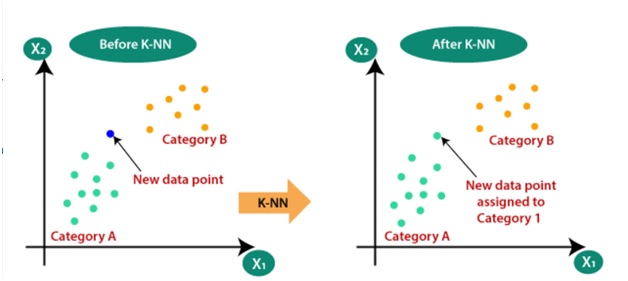
If there are two categories, Category A and Category B, and we have a new data point, x1, which category does this data point belong in? To address this type of problem, we need a K-NN algorithm. K-NN makes determining the category or class of a given dataset simple. Consider the diagram below:

How does K-NN function?

The following algorithm can be used to describe how the K-NN works:

Step 1: Decide on the neighbors’ K-numbers.

Step 2: Calculate the Euclidean distance between K neighbors.

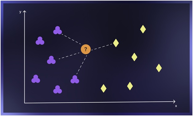
Step 3: Based on the determined Euclidean distance, select the K closest neighbors.

Step 4: Count the number of data points in every part among these k neighbors.

Step 5: Assign the fresh data points to the category where the neighbor count is highest.

Step 6: Our model is complete.

Read our recent article to know whether machine learning is a subset of deep learning.

The kNN algorithm in detail

Give a practice set

A model is trained using a set of labeled data called a training set. You can either use the labeled databases found in open sources like this one or manually label data to generate the training set. A decent rule of thumb is to use about 75% of the data for training and 25% for testing.

K-nearest Neighbors search

Finding a record’s k-nearest neighbors entails locating the records that share the most characteristics with it. This process is often referred to as distance computation or similarity search.

Classify the points

In classification problems, the algorithm chooses a class label by a majority vote, which means that the label that appears more frequently in neighbors is used. The average is used to find the k-nearest neighbors in regression situations. The model outputs the findings following the completion of the aforementioned processes. 

As we employ discrete values in classification issues, the output would be descriptive, such as “likes bright colors,” for example.

Continuous values are used for regression problems, hence a floating-point number would be the output.  How closely the model’s estimates and predictions match the recognized classes in the testing set can be used to gauge how accurate the results are.

How can the k value in the k-neighbors classifier be calculated?

You can increase the model’s accuracy to its highest level by using the ideal k value. However, this process is never easy.

Finding the k value that produces the best results on the testing set is the simplest solution. The steps we take are below:

1. 1. Pick a random value for k. In actual use, k is typically selected at random from 3 to 10, but there are no set guidelines. Decision boundaries become unstable at low values of k. Although improved metrics aren’t usually the result, decision boundaries are frequently smoothed when k is big. So it’s always a matter of trying and failing.
   2. Test out several k values and observe how accurate they are on the testing set.
   3. Implement the model using k with the lowest error rate.

Selecting k in more complex situations

We need to come up with new, time-efficient, and cost-effective ways to calculate k when there are anomalies or a lot of neighbors that are close to an unknown place.

The major constraints are connected to processing resources: the cost of suitable k selection increases with the number of objects in the dataset. Additionally, when working with large datasets, we typically use a multiparameter optimization configuration. By selecting the appropriate k in the meta-training process, we hope to maximize model quality while also accelerating model inference. Inference time increases as k increases, which may be problematic for huge data sets.

We outline several sophisticated strategies for choosing k that work well in certain situations below.

• • Square root method

The square root of the total number of samples in the training dataset can be used to determine the ideal K value. For the best K value, choose an error plot or an accuracy plot. KNN works well with classes that have several labels, but it can struggle with structures that have a lot of outliers, in which case you’ll need to employ alternative techniques.

• • Cross-validation technique (Elbow method)

Start with k=1, then carry out cross-validation (5 to 10 fold) and assess the correctness. These numbers are widely used because they strike a good compromise between computing demands and the need for statistical validity. Till you have consistent results, keep performing the same actions. The error often decreases as k increases, stabilizes, and then starts to increase once more. At the start of the stable zone is where the ideal k is located.

Do you know the difference between data science and machine learning? Just click here to know them in detail.

The k-distance calculation method

The K-distance is the separation between a specified query point and a set of data points. We must choose a distance measure in order to calculate it.

Below are descriptions of some of the most used metrics.

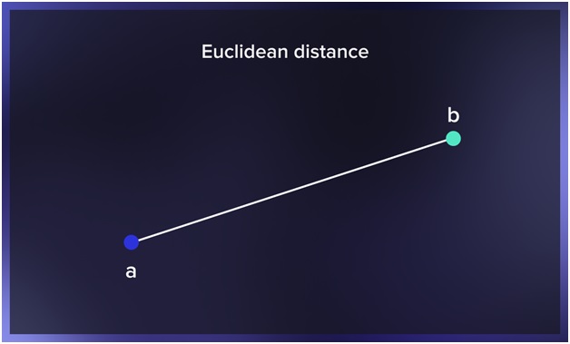
Euclidean Distance

The length of the section of a straight line that connects two points is known as their Euclidean distance. When comparing real-valued vectors, this most used distance metric is used.

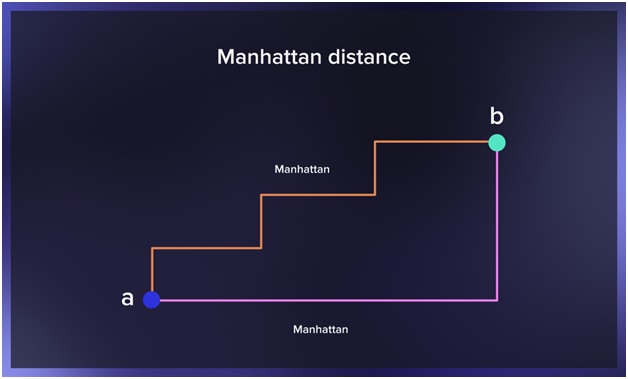
Manhattan’s distance

The total of the absolute differences between each point’s x and y coordinates is the Manhattan distance between the two points. It is sometimes referred to as the taxicab distance and is used to calculate the shortest distance between two points in a city by adding the lengths of each interval.

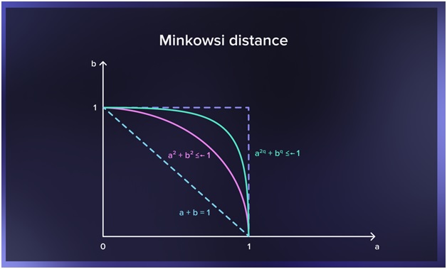
Minkowski distance

The Manhattan and Euclidean distances are generalized by the Minkowski distance. It has an “order” parameter that enables the calculation of various distance metrics. A normed vector space’s Minkowski distance denotes the separation of two points.

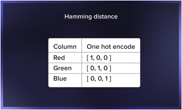
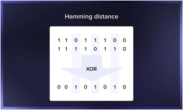
Hamming Distance

Two binary vectors are compared using the Hamming distance method (also called data strings or bitstrings). Data must first be converted into a binary system before it can be calculated.

K-nearest Neighbors in Machine Learning with Python

Let’s examine the classifier’s actual operation.

First Step

1. 1. import numpy as np
   2. from typing import Tuple
   3. def generate_data(center_scale: float, cluster_scale: float, class_counts: np.ndarray,
   4. seed: int = 42) -> Tuple[np.ndarray, np.ndarray]:
   5. np.random.seed(seed)
   6. points, classes = [], []
   7. for class_index, class_count in enumerate(class_counts):
   8. current_center = np.random.normal(scale=center_scale, size=(1, 2))
   9. current_points = np.random.normal(scale=cluster_scale, size=(class_count, 2)) + current_center
   10. current_classes = np.ones(class_count, dtype=np.int64) * class_index
   11. points.append(current_points)
   12. classes.append(current_classes)
   13. points = np.concatenate(points)
   14. classes = np.concatenate(classes)
   15. return points, classes
   16. points, classes = generate_data(2, 0.75, [40, 40, 40], seed=42)
   17. You can execute the following code to plot the data that was generated:
   18. import matplotlib.pyplot as plt
   19. plt.style.use(‘bmh’)
   20. def plot_data(points: np.ndarray, classes: np.ndarray) -> None:
   21. fig, ax = plt.subplots(figsize=(5, 5), dpi=150)
   22. scatter = ax.scatter(x=points[:, 0], y=points[:, 1], c=classes, cmap=’prism’, edgecolor=’black’)
   23. legend = ax.legend(*scatter.legend_elements(), loc=”lower left”, title=”Classes”)
   24. ax.add_artist(legend)
   25. ax.set_title(“Generated dataset”)
   26. ax.set_xticks([])
   27. ax.set_yticks([])
   28. plt.show()
   29. plot_data(points, classes)

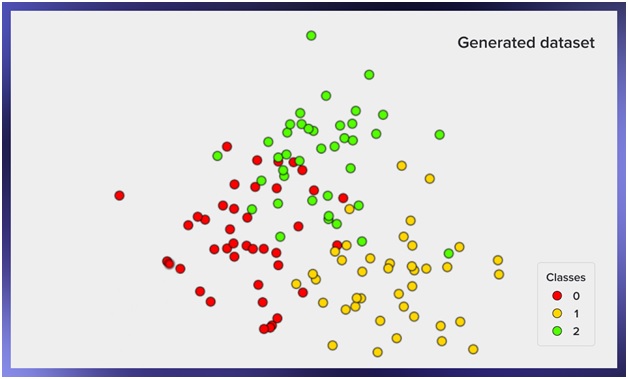
Here is an instance of the image that this code produces:

How to separate training samples from test samples?

Now, we have a group of objects that have been labeled and are individually associated with a class. This set must be divided into a training set and a test set. For this, the following code is implemented:

1. 1. from sklearn.model_selection import train_test_split
   2. points_train, points_test, classes_train, classes_test = train_test_split(
   3.     points, classes, test_size=0.3
   4. )

Implementation of a Classifier

Having a training sample, we can now put the classification algorithm into practice:

1. 1. from collections import Counter
   2. def classify_knn(
   3. points_train: np.ndarray,
   4. classes_train: np.ndarray,
   5. points_test: np.ndarray,
   6. num_neighbors: int
   7. -> np.ndarray:
   8.  classes_test = np.zeros(points_test.shape[0], dtype=np.int64)
   9. for index, test_point in enumerate(points_test):
   10. distances = np.linalg.norm(points_train – test_point, ord=2, axis=1)
   11. neighbors = np.argpartition(distances, num_neighbors)[:num_neighbors]
   12. neighbors_classes = classes_train[neighbors]
   13. test_point_class = Counter(neighbors_classes).most_common(1)[0][0]
   14. classes_test[index] = test_point_class
   15. return classes_test
   16. classes_predicted = classify_knn(points_train, classes_train, points_test, 3)

Execution examples

We can now assess how effectively our classifier performs. In order to achieve this, we produce data, divide it into a training set and a test set, classify the objects in the test set, and then contrast the actual value of the classes in the test set with the value obtained from the classification:

1. 1. def accuracy(classes_true, classes_predicted):
   2. return np.mean(classes_true == classes_predicted)
   3. knn_accuracy = accuracy(classes_test, classes_predicted)
   4. #> knn_accuracy
   5. #  0.8055555555555556

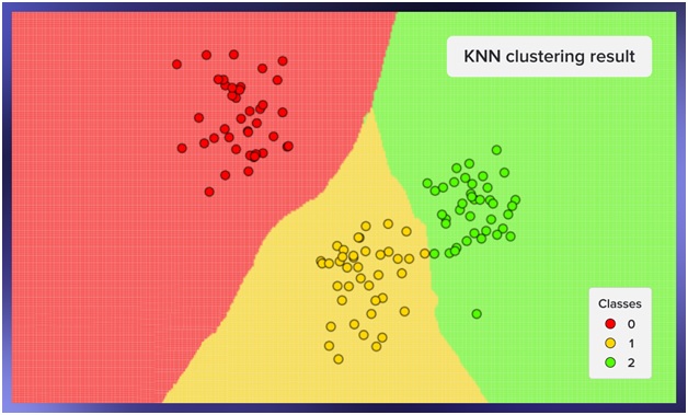
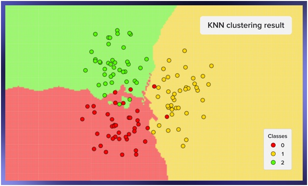
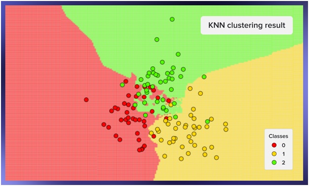
We can now display the classifier’s work graphically. In the images below, we used three classes, each with 40 elements, and the algorithm’s value of k was set to 3.

We can use the following code to make these graphics:

1. 1. def knn_prediction_visualisation(
   2. points: np.ndarray,
   3. classes: np.ndarray,
   4. num_neighbors: int
   5. -> None:
   6. x_min, x_max = points[:, 0].min() – 1, points[:, 0].max() + 1
   7. y_min, y_max = points[:, 1].min() – 1, points[:, 1].max() + 1
   8. step = 0.05
   9. mesh_test_x, mesh_test_y = np.meshgrid(
   10. np.arange(x_min, x_max, step), np.arange(y_min, y_max, step)
   11. )
   12. points_test = np.stack([mesh_test_x.ravel(), mesh_test_y.ravel()], axis=1)
   13. classes_predicted = classify_knn(points, classes, points_test, num_neighbors)
   14. mesh_classes_predicted = classes_predicted.reshape(mesh_test_x.shape)
   15. fig, ax = plt.subplots(figsize=(5, 5), dpi=150)
   16. ax.pcolormesh(mesh_test_x, mesh_test_y, mesh_classes_predicted,
   17. shading=’auto’, cmap=’prism’, alpha=0.4)
   18. scatter = ax.scatter(x=points[:, 0], y=points[:, 1], c=classes,
   19. edgecolors=’black’, cmap=’prism’)
   20. legend = ax.legend(*scatter.legend_elements(), loc=”lower left”, title=”Classes”)
   21. ax.set_title(“KNN clustering result”)
   22. ax.set_xticks([])
   23. ax.set_yticks([])
   24. plt.show()
   25. knn_prediction_visualisation(points, classes, 3)

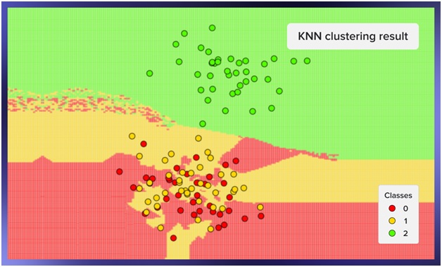
Here are some more clustering examples, starting with the seed 59, moving on to seed 0xdeadbeef, and ending with seed 777 :

Advantages of the KNN Algorithm:

1. 1. • • Easy to Implement
        • It can withstand noisy training data.
        • It may work better if there is a large amount of training data.

Disadvantages of the KNN Algorithm:

1. 1. • • K’s value must always be determined, and sometimes that can be difficult.
        • The high computation cost is caused by the need to determine the separation between each data point for each training sample.

Real-time Applications of KNN

KNN method in automotive production

A new truck and sedan prototype have been created by a carmaker. The business needs to identify which current automobiles on the market most closely resemble the prototypes in order to gauge their prospects of success. Their “closest neighbors” are their rival businesses. The automaker must compare the current models and input information like as pricing, horsepower, engine size, wheelbase, curb weight, and fuel tank capacity in order to identify them. Complex multi-featured prototypes are categorized by the kNN algorithm based on how closely they resemble related competitors’ products.

KNN for E-Commerce

K-nearest neighbors are the greatest way to get an online store recommendation system off the ground, but as the dataset grows, more sophisticated methods are typically required. Based on information about client behavior, the algorithm can choose the products that particular customers would want or forecast their behavior. For instance, kNN can determine in a few seconds whether a new visitor is likely to complete a transaction.

KNN for Education Sector

Classifying groups of students based on their behavior and attendance in class is another application of kNN. The k-nearest neighbors analysis can be used to find students who are most likely to drop out or fail their classes early. These insights would enable instructors and course managers to take prompt action to enthuse students and aid in their topic mastery.

Conclusion

The kNN method is well-liked, efficient, and comparatively simple to use and comprehend. For challenging multivariate instances, it may effectively tackle classification and regression tasks. It still ranks among the top machine learning classifiers despite the emergence of many sophisticated rivals.